R tutorial: How to import data into R

Before you can analyze and visualize data, you have to get that data into R. There are various ways to do this, depending on how your data is formatted and where it’s located.

Usually, the function you use to import data depends on the data’s file format. In base R, for example, you can import a CSV file with read.csv(). Hadley Wickham created a package called readxl that, as you might expect, has a function to read in Excel files. There’s another package, googlesheets, for pulling in data from Google spreadsheets.

But if you don’t want to remember all that, there’s rio.

The magic of rio

“The aim of rio is to make data file I/O [import/output] in R as easy as possible by implementing three simple functions in Swiss-army knife style,” according to the project’s GitHub page. Those functions are import(), export(), and convert().

So, the rio package has just one function to read in many different types of files: import(). If you import("myfile.csv"), it knows to use a function to read a CSV file. import("myspreadsheet.xlsx") works the same way. In fact, rio handles more than two dozen formats including tab-separated data (with the extension .tsv), JSON, Stata, and fixed-width format data (.fwf).

Once you’ve analyzed your data, if you want to save the results as a CSV, Excel spreadsheet, or other formats, rio’s export() function can handle that.

If you don’t already have the rio package on your system, install it now with install.packages("rio").

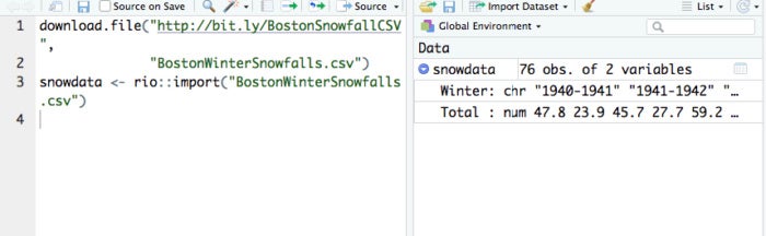
I’ve set up some sample data with Boston winter snowfall data. You could head to http://bit.ly/BostonSnowfallCSV and right-click to save the file as BostonWinterSnowfalls.csv in your current R project working directory. But one of the points of scripting is to replace manual work—tedious or otherwise—with automation that is easy to reproduce. Instead of clicking to download, you can use R’s download.file function with the syntax download.file("url", "destinationFileName.csv"):

download.file("http://bit.ly/BostonSnowfallCSV",
   "BostonWinterSnowfalls.csv")

This assumes that your system will redirect from that Bit.ly URL shortcut and successfully find the real file URL, https://raw.githubusercontent.com/smach/NICAR15data/master/BostonWinterSnowfalls.csv. I’ve occasionally had problems accessing web content on old Windows PCs. If you’ve got one of the those and this Bit.ly link isn’t working, you can swap in the actual URL for the Bit.ly link. Another option is upgrading your Windows PC to Windows 10 if possible to see if that does the trick.

If you wish that rio could just import data directly from a URL, in fact it can, and I’ll get to that in the next section. The point of this section is to get practice working with a local file.

Once you have the test file on your local system, you can load that data into an R object called snowdata with the code:

snowdata <- rio::import("BostonWinterSnowfalls.csv")

Note that it’s possible rio will ask you to redownload the file in binary format, in which case you’ll need to run

download.file("http://bit.ly/BostonSnowfallCSV", 
   "BostonWinterSnowfalls.csv", mode='wb')

Make sure to use RStudio’s tab completion options. If you type rio:: and wait, you’ll get a list of all available functions. Type snow and wait, and you should see the full name of your object as an option. Use your up and down arrow keys to move between auto-completion suggestions. Once the option you want is highlighted, press the Tab key (or Enter) to have the full object or function name added to your script.

You should see the object snowdata appear in your environment tab in the RStudio top right pane. (If that top right pane is showing your command History instead of your Environment, select the Environment tab.)

Taylor & Francis Group

snowdata should show that it has 76 “obs.”—observations, or rows—and two variables, or columns. If you click on the arrow to the left of snowdata to expand the listing, you’ll see the two column names and the type of data each column holds. The Winter is character strings and the Total column is numeric. You should also be able to see the first few values of each column in the Environment pane.

Taylor & Francis Group

Click on the word snowdata itself in the Environment tab for a more spreadsheet-like view of your data. You can get that same view from the R console with the command View(snowdata) (that’s got to be a capital V on View—view won’t work). Note: snowdata is not in quotation marks because you are referring to the name of an R object in your environment. In the rio::import command before, BostonWinterSnowfalls.csv is in quotation marks because that’s not an R object; it’s a character string name of a file outside of R.

Taylor & Francis Group

This view has a couple of spreadsheet-like behaviors. Click a column header to have it sort by that column’s values in ascending order; click the same column header a second time to sort in descending order. There’s a search box to find rows matching certain characters.

If you click the Filter icon, you get a filter for each column. The Winter character column works as you might expect, filtering for any rows that contain the characters you type in. If you click in the Total numerical column’s filter, though, older versions of RStudio show a slider while newer ones show a histogram and a box for filtering.

Import a file from the web

If you want to download and import a file from the web, you can do so if it’s publicly available and in a format such as Excel or CSV. Try

snowdata <- rio::import("http://bit.ly/BostonSnowfallCSV",
   format ="csv")

A lot of systems can follow the redirect URL to the file even after first giving you an error message, as long as you specify the format as "csv" because the file name here doesn’t include .csv. If yours won’t work, use the URL https://raw.githubusercontent.com/smach/R4JournalismBook/master/data/BostonSnowfall.csv instead.

rio can also import well-formatted HTML tables from web pages, but the tables have to be extremely well-formatted. Let’s say you want to download the table that describes the National Weather Service’s severity ratings for snowstorms. The National Centers for Environmental Information Regional Snowfall Index page has just one table, very well crafted, so code like this should work:

rsi_description <- rio::import(
   "https://www.ncdc.noaa.gov/snow-and-ice/rsi/",
   format="html")

Note again that you need to include the format, in this case format="html" . because the URL itself doesn’t give any indication as to what kind of file it is. If the URL included a file name with an .html extension, rio would know.

In real life, though, Web data rarely appears in such neat, isolated form. A good option for cases that aren’t quite as well crafted is often the htmltab package. Install it with install.packages("htmltab"). The package’s function for reading an HTML table is also called htmltab. But if you run this:

library(htmltab)
citytable <- htmltab("https://en.wikipedia.org/wiki/List_of_United_States_cities_by_population")
str(citytable)

you see that you don’t have the correct table, because the data frame contains one object. Because I didn’t specify which table, it pulled the first HTML table on the page. That didn’t happen to be the one I want. I don’t feel like importing every table on the page until I find the right one, but fortunately I have a Chrome extension called Table Capture that lets me view a list of the tables on a page.

The last time I checked, table 5 with more than 300 rows was the one I wanted. If that doesn’t work for you now, try installing Table Capture on a Chrome browser to check which table you want to download.

I’ll try again, specifying table 5 and then seeing what column names are in the new citytable. Note that in the following code, I put the citytable <- htmltab() command onto multiple lines. That’s so it didn’t run over the margins—you can keep everything on a single line. If the table number has changed since this article was posted, replace which = 5 with the correct number.

Instead of using the page at Wikipedia, you can replace the Wikipedia URL with the URL of a copy of the file I created. That file is at http://bit.ly/WikiCityList. To use that version, type bit.ly/WikiCityList into a browser, then copy the lengthy URL it redirects to and use that instead of the Wikipedia URL in the code below:

library(htmltab)
citytable <- htmltab("https://en.wikipedia.org/wiki/List_of_United_States_cities_by_population",
which = 5)
colnames(citytable)

How did I know which was the argument I needed to specify the table number? I read the htmltab help file using the command ?htmltab. That included all available arguments. I scanned the possibilities, and “which a vector of length one for identification of the table in the document” looked right.

Note, too, that I used colnames(citytable) instead of names(citytable) to see the column names. Either will work. Base R also has the rownames() function.

Anyway, those table results are a lot better, although you can see from running str(citytable) that a couple of columns that should be numbers came in as character strings. You can see this both by the chr next to the column name and quotation marks around values like 8,550,405.

This is one of R’s small annoyances: R generally doesn’t understand that 8,550 is a number. I dealt with this problem myself by writing my own function in my own rmiscutils package to turn all those “character strings” that are really numbers with commas back into numbers. Anyone can download the package from GitHub and use it.

The most popular way to install packages from GitHub is to use a package called devtools. devtools is an extremely powerful package designed mostly for people who want to write their own packages, and it includes a few ways to install packages from other places besides CRAN. However, devtools usually requires a couple of extra steps to install compared to a typical package, and I want to leave annoying system-admin tasks until absolutely necessary.

However, the pacman package also installs packages from non-CRAN sources like GitHub. If you haven’t yet, install pacman with install.packages("pacman").

pacman’s p_install_gh("username/packagerepo") function installs from a GitHub repo.

p_load_gh("username/packagerepo") loads a package into memory if it already exists on your system, and it first installs then loads a package from GitHub if the package doesn’t exist locally.

My rmisc utilities package can be found at smach/rmiscutils. Run pacman::p_load_gh("smach/rmiscutils") to install my rmiscutils package.

Note: An alternative package for installing packages from GitHub is called remotes, which you can install via install.packages("remotes"). Its main purpose is to install packages from remote repositories such as GitHub. You can look at the help file with help(package="remotes").

And, possibly the slickest of all is a package called githubinstall. It aims to guess the repo where a package resides. Install it via install.packages("githubinstall"); then you can install my rmiscutils package using githubinstall::gh_install_packages("rmiscutils"). You are asked if you want to install the package at smach/rmisutils (you do).

Now that you’ve installed my collection of functions, you can use my number_with_commas() function to change those character strings that should be numbers back into numbers. I strongly suggest adding a new column to the data frame instead of modifying an existing column—that’s good data analysis practice no matter what platform you’re using.

In this example, I’ll call the new column PopEst2017. (If the table has been updated since, use appropriate column names.)

library(rmiscutils)
citytable$PopEst2017 <- number_with_commas(citytable$`2017 estimate`)

My rmiscutils package isn’t the only way to deal with imported numbers that have commas, by the way. After I created my rmiscutils package and its number_with_commas() function, the tidyverse readr package was born. readr also includes a function that turns character strings into numbers, parse_number().

After installing readr, you could generate numbers from the 2017 estimate column with readr:

citytable$PopEst2017 <- readr::parse_number(citytable$`2017 estimate`)

One advantage of readr::parse_number() is that you can define your own locale() to control things like encoding and decimal marks, which may be of interest to non-US-based readers. Run ?parse_number for more information.

Note: If you didn’t use tab completion for the 2017 estimate column, you might have had a problem with that column name if it has a space in it at the time you are running this code. In my code above, notice there are backward single quote marks (`) around the column name. That’s because the existing name had a space in it, which you’re not supposed to have in R. That column name has another problem: It starts with a number, also generally an R no-no. RStudio knows this, and automatically adds the needed back quotes around the name with tab autocomplete.

Bonus tip: There’s an R package (of course there is!) called janitor that can automatically fix troublesome column names imported from a non-R-friendly data source. Install it with install.packages("janitor"). Then, you can create new clean column names using janitor’s clean_names() function.

Now, I’ll create an entirely new data frame instead of altering column names on my original data frame, and run janitor’s clean_names() on the original data. Then, check the data frame column names with names():

citytable_cleaned <- janitor::clean_names(citytable)
names(citytable_cleaned)

You see the spaces have been changed to underscores, which are legal in R variable names (as are periods). And, all column names that used to start with a number now have an x at the beginning.

If you don’t want to waste memory by having two copies of essentially the same data, you can remove an R object from your working session with rm() function: rm(citytable).

Import data from packages

There are several packages that let you access data directly from R. One is quantmod, which allows you to pull some US government and financial data directly into R.

Another is the aptly named weatherdata package on CRAN. It can pull data from the Weather Underground API, which has information for many countries around the world. 

The rnoaa package, a project from the rOpenSci group, taps into several different US National Oceanic and Atmospheric Administration data sets, including daily climate, buoy, and storm information.

If you are interested in state or local government data in the US or Canada, you may want to check out RSocrata to see if an agency you’re interested in posts data there. I’ve yet to find a complete list of all available Socrata data sets, but there’s a search page at https://www.opendatanetwork.com. Be careful, though: There are community-uploaded sets along with official government data, so check a data set’s owner and upload source before relying on it for more than R practice. “ODN Dataset” in a result means it’s a file uploaded by someone in the general public. Official government data sets tend to live at URLs like https://data.CityOrStateName.gov and https://data.CityOrStateName.us.

For more data-import packages, see my searchable chart at http://bit.ly/RDataPkgs. If you work with US government data, you might be particularly interested in censusapi and tidycensus, both of which tap into US Census Bureau data. Other useful government data packages include eu.us.opendata from the US and European Union governments to make it easier to compare data in both regions, and cancensus for Canadian census data.

When the data’s not ideally formatted

In all these sample data cases, the data has been not only well-formatted, but ideal: Once I found it, it was perfectly structured for R. What do I mean by that? It was rectangular, with each cell having a single value instead of merged cells. And the first row had column headers, as opposed to, say, a title row in large font across multiple cells in order to look pretty—or no column headers at all.

Dealing with untidy data can, unfortunately, get pretty complicated. But there are a couple of common issues that are easy to fix.

Beginning rows that aren’t part of the data. If you know that the first few rows of an Excel spreadsheeet don’t have data you want, you can tell rio to skip one or more lines. The syntax is rio::import("mySpreadsheet.xlsx", skip=3) to exclude the first three rows. skip takes an integer.

There are no column names in the spreadsheet. The default import assumes the first row of your sheet is the column names. If your data doesn’t have headers, the first row of your data may end up as your column headers. To avoid that, use rio::import("mySpreadsheet.xlsx", col_names = FALSE) so R will generate default headers of X0, X1, X2, and so on. Or, use a syntax such as rio::import("mySpreadsheet.xlsx", col_names = c("City", "State", "Population")) to set your own column names.

If there are multiple tabs in your spreadsheet, the which argument overrides the default of reading in the first worksheet. rio::import("mySpreadsheet.xlsx", which = 2) reads in the second worksheet.

What’s a data frame? And what can you do with one?

rio imports a spreadsheet or CSV file as an R data frame. How do you know whether you’ve got a data frame? In the case of snowdata, class(snowdata) returns the class, or type, of object it is. str(snowdata) also tells you the class and adds a bit more information. Much of the info you see with str() is similar to what you saw for this example in the RStudio environment pane: snowdata has 76 observations (rows) and two variables (columns).

Data frames are somewhat like spreadsheets in that they have columns and rows. However, data frames are more structured. Each column in a data frame is an R vector, which means that every item in a column has to be the same data type. One column can be all numbers and another column can be all strings, but within a column, the data has to be consistent.

If you’ve got a data frame column with the values 5, 7, 4, and “value to come,” R will not simply be unhappy and give you an error. Instead, it will coerce all your values to be the same data type. Because “value to come” can’t be turned into a number, 5, 7, and 4 will end up being turned into character strings of "5", "7", and "4". This isn’t usually what you want, so it’s important to be aware of what type of data is in each column. One stray character string value in a column of 1,000 numbers can turn the whole thing into characters. If you want numbers, make sure you have them!

R does have a ways of referring to missing data that won’t screw up the rest of your columns: NA means “not available.”

Data frames are rectangular: Each row has to have the same number of entries (although some can be blank), and each column has to have the same number of items.

Excel spreadsheet columns are typically referred to by letters: Column A, Column B, etc. You can refer to a data frame column with its name, by using the syntax dataFrameName$columnName. So, if you type snowdata$Total and press Enter, you see all the values in the Total column, as shown in the figure below. (That’s why when you run the str(snowdata) command, there’s a dollar sign before the name of each column.)

Taylor & Francis Group

A reminder that those bracketed numbers at the left of the listing aren’t part of the data; they’re just telling you what position each line of data starts with. [1] means that line starts with the first item in the vector, [10] the tenth, etc.

RStudio tab completion works with data frame column names as well as object and function names. This is pretty useful to make sure you don’t misspell a column name and break your script—and it also saves typing if you’ve got long column names.

Type snowdata$ and wait, then you see a list of all the column names in snowdata.

It’s easy to add a column to a data frame. Currently, the Total column shows winter snowfall in inches. To add a column showing totals in meters, you can use this format:

snowdata$Meters <- snowdata$Total * 0.0254

The name of the new column is on the left, and there’s a formula on the right. In Excel, you might have used =A2 * 0.0254 and then copied the formula down the column. With a script, you don’t have to worry about whether you’ve applied the formula properly to all the values in the column.

Now look at your snowdata object in the Environment tab. It should have a third variable, Meters.

Because snowdata is a data frame, it has certain data-frame properties that you can access from the command line. nrow(snowdata) gives you the numbers of rows and ncol(snowdata) the number of columns. Yes, you can view this in the RStudio environment to see how many observations and variables there are, but there will probably be times when you’ll want to know this as part of a script. colnames(snowdata) or names(snowdata) gives you the name of snowdata columns. rownames(snowdata) give you any row names (if none were set, it will default to character strings of the row number such as "1", "2", "3", etc.).

Some of these special dataframe functions, also known as methods, not only give you information but let you change characteristics of the data frame. So, names(snowdata) tells you the column names in the data frame, but

names(snowdata) <- c("Winter", "SnowInches", "SnowMeters")

changes the column names in the data frame.

You probably won’t need to know all available methods for a data frame object, but if you’re curious, methods(class=class(snowdata)) displays them. To find out more about any method, run the usual help query with a question mark, such as ?merge or ?subset.

When a number’s not really a number

ZIP codes are a good example of “numbers” that shouldn’t really be treated as such. Although technically numeric, it doesn’t make sense to do things like add two ZIP codes together or take an average of ZIP codes in a community. If you import a ZIP-code column, R will likely turn it into a column of numbers. And if you’re dealing with areas in New England where ZIP codes start with 0, the 0 will disappear.

I have a tab-delineated file of Boston ZIP codes by neighborhood, downloaded from a Massachusetts government agency, at https://raw.githubusercontent.com/smach/R4JournalismBook/master/data/bostonzips.txt. If I tried to import it with zips <- rio::import("bostonzips.txt"), the ZIP codes would come in as 2118, 2119, etc. and not 02118, 02119, and so on.

This is where it helps to know a little bit about the underlying function that rio’s import() function uses. You can find those underlying functions by reading the import help file at ?import. For pulling in tab-separated files, import uses either fread() from the data.table package or base R’s read.table() function. The ?read.table help says that you can specify column classes with the colClasses argument.

Create a data subdirectory in your current project directory, then download the bostonzips.txt file with

download.file("https://raw.githubusercontent.com/smach/R4JournalismBook/master/data/bostonzips.txt", "data/bostonzips.txt")

If you import this file specifying both columns as character strings, the ZIP codes will come in properly formated:

zips <- rio::import("data/bostonzips.txt", colClasses = 
   c("character”", "character"))
str(zips)

Note that the column classes have to be set using the c() function, c("character", "character"). If you tried colClasses ="character", "character", you’d get an error message. This is a typical error for R beginners, but it shouldn’t take long to get into the c() habit.

A save-yourself-some-typing tip: Writing out c("character", "character") isn’t all that arduous; but if you’ve got a spreadsheet with 16 columns where the first 14 need to be character strings, this can get annoying. R’s rep() function can help. rep(), as you might have guessed, repeats whatever item you give it however many times you tell it to, using the format rep(myitem, numtimes). rep("character", 2) is the same as c("character", "character"), so colClasses = rep("character", 2) is equivalent to colClasses = c("character", "character") . And, colClasses = c(rep("character", 14), rep("numeric", 2)) sets the first 14 columns as character strings and the last two as numbers. All the names of column classes here need to be in quotation marks because names are character strings.

I suggest you play around a little with rep() so you get used to the format, since it’s a syntax that other R functions use, too.

Easy sample data

R comes with some built-in data sets that are easy to use if you want to play around with new functions or other programming techniques. They’re also used a lot by people teaching R, since instructors can be sure that all students are starting off with the same data in exactly the same format.

Type data() to see available built-in data sets in base R and whatever installed packages are currently loaded. data(package = .packages(all.available = TRUE)) from base R displays all possible data sets from packages that are installed in your system, whether or not they’re loaded into memory in your current working session.

You can get more information about a data set the same way you get help with functions: ?datasetname or help("datasetname"). mtcars and iris are among those I’ve seen used very often.

If you type mtcars, the entire mtcars data set prints out in your console. You can use the head() function to look at the first few rows with head(mtcars).

You can store that data set in another variable if you want, with a format like cardata <- mtcars.

Or, running the data function with the data set name, such as data(mtcars), loads the data set into your working environment.

One of the most interesting packages with sample data sets for journalists is the fivethirtyeight package, which has data from stories published on the FiveThirtyEight.com website. The package was created by several academics in consultation with FiveThirtyEight editors; it is designed to be a resource for teaching undergraduate statistics.

Prepackaged data can be useful—and in some cases fun. In the real world, though, you may not be using data that’s quite so conveniently packaged.

Create a data frame manually in R

Chances are, you’ll often be dealing with data that starts off outside of R and you import from a spreadsheet, CSV file, API, or other source. But sometimes you might just want to type a small amount of data directly into R, or otherwise create a data frame manually. So let’s take a quick look at how that works.

R data frames are assembled column by column by default, not one row at a time. If you wanted to assemble a quick data frame of town election results, you could create a vector of candidate names, a second vector with their party affiliation, and then a vector of their vote totals:

candidates <- c("Smith", "Jones", "Write-ins", "Blanks")
party <- c("Democrat", "Republican", "", "")
votes <- c(15248, 16723, 230, 5234)

Remember not to use commas in your numbers, like you might do in Excel.

To create a data frame from those columns, use the data.frame() function and the synatx data.frame(column1, column2, column3).

myresults <- data.frame(candidates, party, votes)

Check its structure with str():

str(myresults)

While the candidates and party vectors are characters, the candidates and party data frame columns have been turned into a class of R objects called factors. It’s a bit too in-the-weeds at this point to delve into how factors are different from characters, except to say that

1. Factors can be useful if you want to order items in a certain, nonalphabetical way for graphing and other purposes, such as Poor is less than Fair is less than Good is less than Excellent.
2. Factors can behave differently than you might expect at times. I recommend sticking with character strings unless you have a good reason to specifically want factors.

You can keep your character strings intact when creating data frames by adding the argument stringsAsFactors = FALSE:

myresults <- data.frame(candidates, party, votes, 
   stringsAsFactors = FALSE)
str(myresults)

Now, the values are what you expected.

There’s one more thing I need to warn you about when creating data frames this way: If one column is shorter than the other(s), R will sometimes repeat data from the shorter column—whether or not you want that to happen.

Say, for example, you created the election results columns for candidates and party but only entered votes results for Smith and Jones, not for Write-ins and Blanks. You might expect the data frame would show the other two entries as blank, but you’d be wrong. Try it and see, by creating a new votes vector with just two numbers, and using that new votes vector to create another data frame:

votes <- c(15248, 16723)
myresults2 <- data.frame(candidates, party, votes)
str(myresults2)

That’s right, R reused the first two numbers, which is definitely not what you’d want. If you try this with three numbers in the votes vector instead of two or four, R would throw an error. That’s because each entry couldn’t be recycled the same number of times.

If by now you’re thinking, “Why can’t I create data frames that don’t change strings into factors automatically? And why do I have to worry about data frames reusing one column’s data if I forget to complete all the data?” Hadley Wickham had the same thought. His tibble package creates an R class, also called tibble, that he says is a “modern take on data frames. They keep the features that have stood the test of time, and drop the features that used to be convenient but are now frustrating.”

If this appeals to you, install the tibble package if it’s not on your system and then try to create a tibble with

myresults3 <- tibble::tibble(candidates, party, votes)

and you’ll get an error message that the votes column needs to be either 4four items long or one item long (tibble() will repeat a single item as many times as needed, but only for one item).

Put the votes column back to four entries if you’d like to create a tibble with this data:

library(tibble)
votes <- c(15248, 16723, 230, 5234)
myresults3 <- tibble(candidates, party, votes)
str(myresults3)

It looks similar to a data frame—in fact, it is a data frame, but with some special behaviors, such as how it prints. Also notice that the candidates column is character strings, not factors.

If you like this behavior, go ahead and use tibbles. However, given how prevelant conventional data frames remain in R, it’s still important to know about their default behaviors.

Exporting data

Often after you’ve wrangled your data in R, you want to save your results. Here are some of the ways to export your data that I tend to use most:

Save to a CSV file with rio::export(myObjectName, file="myFileName.csv") and to an Excel file with rio::export(myObjectName, file="myFileName.xlsx"). rio understands what file format you want based on the extension of the file name. There are several other available formats, including .tsv for tab-separated data, .json for JSON, and .xml for XML.

Save to an R binary object that makes it easy to load back into R in future sessions. There are two options.

Generic save() saves one or more objects into a file, such as save(objectName1, objectName2, file="myfilename.RData"). To read this data back into R, you just use the command load("myfilename.RData") and all the objects return with the same names in the same state they had before.

You can also save a single object into a file with saveRDS(myobject, file="filename.rds"). The logical assumption is that loadRDS would read the file back in, but instead the command is readRDS—and in this case, just the data has been stored, not the object name. So, you need to read the data into a new object name, such as mydata <- readRDS("filename.rds").

There’s a third way of saving an R object specifically for R: generating the R commands that would recreate the object instead of the object with final results. The base R functions for generating an R file to recreate an object are dput() or dump(). However, I find rio::export(myobject, "mysavedfile.R") even easier to remember.

Finally, there are additional ways to save files that optimize for readability, speed, or compression, which I mention in the additional resources section at the end of this article.

You can also export an R object into your Windows or Mac clipboard with rio: rio::export(myObjectName, format ="clipboard"). And, you can import data into R from your clipboard the same way: rio::import(file ="clipboard").

Bonus: rio’s convert() function lets you—you guessed it—convert one file type to another without having to manually pull the data into and then out of R. See ?convert for more info.

Final point: RStudio lets you click to import a file, without having to write code at all. This isn’t something I recommend until you’re comfortable importing from the command line, beause I think it’s important to understand the code behind importing. But, I admit this can be a handy shortcut.

In the Files tab of RStudio’s lower right pane, navigate to the file you want to import and click it. You’ll see an option to either View File or Import Dataset. Choose Import Dataset to see a dialog that previews the data, lets you modify how the data is imported, and previews the code that will be generated.

Make whatever changes you want and click Import, and your data will be pulled into R.

Additional resources

rio alternatives. While rio is a great Swiss Army knife of file handling, there may be times when you want a bit more control over how your data is pulled into or saved out of R. In addition, there have been times when I’ve had a challenging data file that rio choked on but another package could handle it. Some other functions and packages you may want to explore:

• Base R’s read.csv() and read.table() to import text files (use ?read.csv and ?read.table to get more information). stringsAsFactors = FALSE is needed with these if you want to keep your character strings as character strings. write.csv() saves to CSV.
• rio uses Hadley Wickham’s readxl package for reading Excel files. Another alternative for Excel is openxlsx, which can write to an Excel file as well as read one. Look at the openxlsx package vignettes for information about formatting your spreadsheets as you export.
• Wickham’s readr package is also worth a look as part of the “tidyverse.” readr includes functions to read CSV, tab-separated, fixed-width, web logs, and several other types of files. readr prints out the type of data it has determined for each column—integer, character, double (non-whole numbers), etc. It creates tibbles.

Import directly from a Google spreadsheet. The googlesheets package lets you import data from a Google Sheets spreadsheet, even if it’s private, by authenticating your Google account. The package is available on CRAN; install it via install.packages("googlesheets"). After loading it with library("googlesheets"), read the excellent introductory vignette. At the time of this writing, the intro vignette was available in R at vignette("basic-usage", package="googlesheets"). If you don’t see it, try help(package="googlesheets") and click the User Guides, Package Vignettes and Other Documentation link for available vignettes, or look at the package information on GitHub at https://github.com/jennybc/googlesheets.

Scrape data from Web pages with the rvest package and SelectorGadget browser extension or JavaScript bookmarklet. SelectorGadget helps you discover the CSS elements of data you want to copy that are on an HTML page; then rvest uses R to find and save that data. This is not a technique for raw beginners, but once you’ve got some R experience under your belt, you may want to come back and revisit this. I have some instructions and a video on how to do this at http://bit.ly/Rscraping. RStudio has a webinar available on demand as well.

Alternatives to base R’s save and read functions. If you are working with large data sets, speed may become important to you when saving and loading files. The data.table package has a speedy fread() function, but beware that resulting objects are data.tables and not plain data frames; some behaviors are different. If you want a conventional data frame, you can get one with the as.data.frame(mydatatable) syntax. The data.table package’s fwrite() function is aimed at writing to a CSV file considerably faster than base R’s write.csv().

Two other packages might be of interest for storing and retrieving data. The feather package saves in a binary format that can be read either into R or Python. And, the fst package’s read.fst() and write.fst() offer fast saving and loading of R data frame objects—plus the option of file compression.